Take the shortest route, the one that nature planned
Marcus Aurelius, Meditations
Genetic algorithms are really interesting in my opinion. Not the most efficient, but rather beautiful in the way they work. I especially like them because of the similarities that they share with life. Genetic algorithms are special kind of algorithms that work by modelling how natural selection works in the real world. I shouldn’t need to explain how evolution works, but for the sake of it, here I go. We have several individuals in a population, given their environment, some of the individual are better suited and reproduce, propagating their traits to their offspring. In the process, mutations and other random processes happen that allow for some wiggle room and hopefully improve the offspring fitness to the environment. The cycle continues on and on, with gradual improvement of the individuals that are better adjusted to their environment.
In the genetic algorithm, every step natural selection is simulated to solve a mathematical problem. We have various individuals, that are the potential solutions to the problem we consider. We estimate which individuals are the best potential solutions and we keep them. We then create this artificial mating process wherein we take some characteristic of one individual potential solution and mix it with the characteristics of another individual potential solution. This creates a new generation of individuals… We add some randomness to the offspring, meaning that the new generation can have some differences from the parents, which could make them worse solutions or hopefully better solutions. We repeat the process until we are happy with the result, or we see that the algorithm is converging and doesn’t make progress any more.
Let’s get deeper and consider that the problem we want to solve is the fitting of a polynomial curve over some data. In parallel to me explaining the what a genetic algorithm is, I am going to copy bits and pieces of my own algorithm to show how I did it.
At the start of the problem here, we have the dataset that we want to fit with a polynomial curve. This dataset could come from some measurements, but for the sake of the discussion here, I generate the dataset from a polynomial function. I decide the polynomial function before hand and add some randomness to it (the jitter). This simulates the dataset for the fitting algorithm.
This step, I do in a special function in python:
import random
import numpy as np
import matplotlib.pyplot as plt

def generate_fuzzy_data(coef_list: list, x_boundary: list, jitter=0, show_coefficients=False):
    """
    Function to generate data for the polynomial fitting with some randomness to it
    :param coef_list: [b_0, b_1, b_2, ..., b_n] for a polynome like b_0 + b_1*x + b_2*x^2 + ... + b_n*x^n
    :param x_boundary: [x_min, x_max] to generate data between x_min and x_max
    :param jitter: this is a float, in percent, giving the amount of randomness to add to the polynomial data
    :param show_coefficients: boolean to display the coefficients
    :return: the list of x and the list of the corresponding polynomial values with the added randomness
    """

    data = []
    abscisse = []
    order = len(coef_list)
    start = x_boundary[0]
    stop = x_boundary[1]

    number_of_points = 100  # Keeping this parameter fixed for the moment

    if show_coefficients:
        if coef_list:
            print("Using coefficients:")
            for coef in coef_list:
                print(f"{coef}")

        else:
            print("using random coefficients")
            coef_list = [random.uniform(-1, 1) for _i in range(order)]

    order_list = list(range(order))

    for x in range(number_of_points):
        data.append(0)
        abscisse.append(start+x*(stop-start)/(number_of_points-1))
        for index in range(order):
            data[x] += coef_list[index] * pow(abscisse[x], order_list[index])

    span = (np.max(data) - np.min(data))

    return abscisse, list(map(lambda y: y + span * random.uniform(-jitter/100, jitter/100), data))
This “generate fuzzy data” function takes a coefficient list as input, along with the x boundary for generating the data and a jitter value that controls the amount of randomness that I want. It will output two lists, one containing the x values and the other containing the y values that are the polynomial values with the added randomness.
The fitting is done with a polynomial equation, so we know that this equation is going to be of the form:
b_0 + b_1 x + b_2 x^2 + … + b_n x^nwith b_0, b_1, b_2, … b_n the polynomial coefficients, and n the degree of the polynomial. The goal of the genetic algorithm is to find these b_k coefficients so that the polynomial function that we create with them is as close as possible to the dataset. To do that, we are going to take a random set of coefficients, for instance a set that I will call S1=a_0, a_1, a_2, …, a_n. This set S1 can also be called an individual, or even a chromosome if we want to keep in the “genetic” lingo. In the genetic fitting algorithm, we are going to use several different individuals, that is to say, several sets containing coefficients with various values, different from one individual to the other. This simulates the genetic diversity of a given population. Because of this, I will call the ensemble of individual a population.
The first step of the genetic algorithm is to create a starter population. The user is going to tell how many individual in the population they want, the more the better but also the longer… The algorithm then will create random values for these coefficients. It can be useful to start with coefficients as close as possible to the target, it helps with the convergence of the algorithm, of course. But even totally random numbers will do the trick.
For the Python code, I decided to use a class for the genetic fitting, so I will just give the initialisation step first, along with the function to import the data into the data_x and data_y fields. I also give you the various import that I used in this script. The “generate fuzzy data” is located in another file, that I called addons, so don’t be surprised by this. I also use the “rich” package to display a progress bar during the fitting. It makes the waiting a little more bearable…
import numpy as np
import random
import addons
import matplotlib.pyplot as plt
from rich.progress import track
import time
import statistics


class PolynomialGeneticAlgorithm:
    def __init__(self, fitting_order):
        self.data_x = []
        self.data_y = []
        self.order = fitting_order
        self.population = []
        self.fitness = []

    def load_data(self, data_x, data_y):
        self.data_x = data_x
        self.data_y = data_y
The generation of the population is done by this code inside the PolynomialGeneticAlgorithm class:
class PolynomialGeneticAlgorithm:
...
   def create_population(self, number_of_individual):
        self.population = np.zeros((number_of_individual, self.order), dtype=float)
        for individual in range(number_of_individual):
            for coefficient in range(self.order):
                self.population[individual][coefficient] = random.uniform(-10, 10)
        self.fitness = list(np.zeros(number_of_individual, dtype=float))
I decided to generate the coefficient randomly between -10 and 10, but this really can be set to any other values.
The next step is also important. This is the step where we compute the error in the fitting of the dataset. This is called the fitness and it needs to be evaluated for each individual. For each individual, we are going to take the coefficients, input them in the polynomial equation and for each points in the dataset, compute the error between the data point and the fitting curve. The fitness function is important, taking the correct function can help accelerate the convergence of the algorithm. Here, I took the sum of the square root of the difference between a data point and the fitting curve. Because I wanted to have a large number when the curve is getting better and better fitted, I took the inverse of that sum as the fitness value. Smaller value mean that the curve is not well fitted, larger values mean that it is better fitted. This is the what is performed by the following function:
class PolynomialGeneticAlgorithm:
...
    def get_fitness(self):
        self.fitness = []
        individual_index = 0

        for _ in self.population:
            temp_data = []
            for x in self.data_x:
                temp_value = 0
                for coef in range(self.order):
                    temp_value += self.population[individual_index][coef] * pow(x, coef)
                temp_data.append(temp_value)
            try:
                self.fitness.append(1/(sum([(x1 - x2)**2 for (x1, x2) in zip(temp_data, self.data_y)])))
            except ZeroDivisionError:
                self.fitness.append(99999)
            individual_index += 1
Once all the fitnesses are calculated, we decide to keep a given amount of individuals with the best fitness, that is to say the individuals that give the best fitting result with the curve the closest to the dataset. These individuals are the selected few that will be used to generate the next set of individuals that we are going to call the offsprings. This is what is done by the “select_mating” function:
class PolynomialGeneticAlgorithm:
...
    def select_mating(self, number_of_mates):
        selected = np.zeros((number_of_mates, self.order))
        for i in range(number_of_mates):
            max_fitness = max(self.fitness)
            max_fitness_index = np.where(self.fitness == max_fitness)[0][0]
            selected[i] = self.population[max_fitness_index]
            self.fitness[int(max_fitness_index)] = 0.0
        return selected
And now the fun begins. It is good to have an even number of selected individuals to create pairs of individuals for the “mating” simulation. Let’s focus on a pair of individuals that were selected. They are S1 and S2. S1 is a set (a_0, a_1, a_2, … a_n) and S2 is a set (a’_0, a’_1, a’_2, …, a’_n). The idea of the mating simulation is to generate from these two sets, two more sets of offspring by mixing the values in the set between one another. To do that, we need to decide of a crossover point. This is the moment where we need to think of the sets as chromosomes in the discussion. Each set is the same length, n. We need to decide a crossover point (index k) that is comprised between 0 and n, k in ]0,n[. This crossover point can either be chosen at random or fixed at some point, in the middle of the set.
Here is the code corresponding to the crossover step:
class PolynomialGeneticAlgorithm:
...
    def crossover(self, parents, random_crossover=False):
        offspring = np.zeros((len(parents), self.order), dtype=float)
        couples = addons.create_random_couples(parents.tolist())
        index = 0
        for couple in couples:
            if len(couple) == 2:
                if random_crossover:
                    crossover_point = np.uint8(np.random.uniform(1, self.order))
                else:
                    crossover_point = np.uint8(self.order / 2)
                offspring[index] = couple[0][:crossover_point] + couple[1][crossover_point:]
                offspring[index+1] = couple[1][:crossover_point] + couple[0][crossover_point:]
                index += 2
            else:
                # There are no mate for this individual, so it is skipped.
                offspring[index] = couple[0]
                index += 1

        return offspring
I use in this bit of code another function called “create_random_couples”, from outside this script, that is going to select randomly the selected parents for the mating. This way, I don’t make just the best solutions mate with one another and have the less efficient solutions mate with one another. It is all done randomly. Here is that function:
def create_random_couples(list_of_elements:list):
    random.shuffle(list_of_elements)
    index = 0
    result = []
    for _ in range(len(list_of_elements) // 2):
        result.append([list_of_elements[index], list_of_elements[index+1]])
        index += 2
    if len(list_of_elements) % 2:
        result.append([list_of_elements[-1]])
    return result
Little pause here. I wrote earlier that I liked the genetic algorithm because it simulates life. And here is the precision about this. The crossover process is something that really happens between chromosomes. In each one of our cells there are two copies of each chromosomes, one from the father, one from the mother. That is what you see when you do the human caryotype [1]. You see 23 pairs of chromosomes, 46 total. 23 coming from the mother, 23 coming from the father. During the fabrication of the gametes, that is to say the eggs or the sperm cells, the chromosomes go through the meiosis step, where they first duplicate, forming the famous x shape that we see when we picture chromosomes. They then intertwine, and eventually one bit of the information encoded in the chromosome coming from the father gets in the chromosome coming from the mother, or vice-versa. This step is called the cross-over [2]. And this is what we are simulating here in our algorithm…
Back to the algorithm itself. We have the crossover point k. For this pair of chromosome, we are going to generate two offspring: a set S3 which is (a_0, a_1, … , a_k-1, a_k, a’_k+1, … a’_n) and S4 which is (a’_0, a’_1, … , a’_k-1, a’_k, a_k+1, … a_n).
Next step is equally important. Because simply moving values from one set to the other is not enough to converge toward a solution. The thing missing is the mutation. That is to say that each offspring is going to have a “risk” of seeing a change in the values that compose its set. Again, the whole game is to decide how much we want to make the value change, and what mutation rate we want to have. If the mutation rate is too high, it could cause the convergence to fail, and the offspring to being worse than the parents every time. If the mutation rate is too slow, well, it would take longer to reach the convergence of course. So there is an optimal value there, which depends on the context unfortunately. Here, in my code, I decided to play with the mutation rate and the mutation range, to optimize the mutation step. Here it is:
class PolynomialGeneticAlgorithm:
...
    def mutation(self, population, mutation_range=1, mutation_rate=0.5):
        to_mutate = np.zeros(population.shape)
        for i in range(population.shape[0]):
            for j in range(population.shape[1]):
                to_mutate[i][j] = random.uniform(-mutation_range/2, mutation_range/2) if random.uniform(0, 1) > \
                                                                                         mutation_rate else 0

        return population + to_mutate
Finally, we can regroup the parent set and the offspring set into a new population. The loop is closed, and we can start to measure the fitness of each individual in the population to decide which is the closest to the dataset. Repeat the loop for a few hundred times and you will converge into a local and eventually global solution given the mutation range and rate.
Here is the code doing this loop. This time, outside the class, of course. We first need to create an instance of the PolynomialGeneticAlgorithm class, create the data and then make the actual loop:
gen = PolynomialGeneticAlgorithm(5)

# Polynomial parameters for the generation of the simulated random data
polynomial_coefs = [-2.2, 6.4, 1.3, -0.5, 0.2]
data_boundary_x = [-4, 5]

data_test_abs, data_test = addons.generate_fuzzy_data(polynomial_coefs, data_boundary_x, jitter=10)

gen.load_data(data_x=data_test_abs, data_y=data_test)

# Create a population consisting of 32 individuals
gen.create_population(32)

offsprings = []
fitness_result = []
fitness_timing = []
select_mating_timing = []
offspring_timing = []
mutation_timing = []
average_fitness_result = []

# Loop for N times. This needs to be adjusted until the result converges.
for _ in track(range(3000), description="Iterating"):
    start = time.perf_counter()
    gen.get_fitness()
    fitness_timing.append(time.perf_counter()-start)

    fitness_result.append(max(gen.fitness))
    average_fitness_result.append(statistics.mean(gen.fitness))

    start = time.perf_counter()
    mates = gen.select_mating(16)
    select_mating_timing.append(time.perf_counter()-start)

    start = time.perf_counter()
    offsprings = gen.crossover(mates, random_crossover=True)
    offspring_timing.append(time.perf_counter()-start)

    start = time.perf_counter()
    mutants = gen.mutation(offsprings, mutation_range=2, mutation_rate=0.1)
    mutation_timing.append(time.perf_counter()-start)

    gen.population = np.vstack([mates, mutants])
And there it is. It is definitely not the most efficient algorithm for polynomial fitting that there is, but I like it quite a lot. It is also not restricted to polynomial fitting at all. This is actually the other beauty of this algorithm… As long as there are parameters to vary, it can work. Say you want to fit a dataset with a function like a_0+a_1*\sin(a_2*x)+a_2\cos(a_3*x)+a_4*x+\sin(a_5*x), then it is possible. The only thing to perform is create the right function for the fitness test. That is all. Given enough time, it will converge…
And finally for the display:
fig2, ax = plt.subplots()
ax.scatter(gen.data_x, gen.data_y, color="C0", label="Original data used for the fitting", marker="+")

data_perfect_x, data_perfect_y = addons.generate_fuzzy_data(polynomial_coefs, data_boundary_x, jitter=0)
ax.plot(data_perfect_x, data_perfect_y, color="C2", label="Original data with no randomness")

# find the best result in the population
gen.get_fitness()
winner = gen.population[gen.fitness.index(max(gen.fitness))]

fitting_data_x, fitting_data_y = addons.generate_fuzzy_data([winner[0], winner[1], winner[2], winner[3], winner[4]],
                                                                data_boundary_x)

ax.plot(fitting_data_x, fitting_data_y, "C1", label="Fitting result")
ax.legend()
ax.set_title("Fitting over the dataset")
ax.set_xlabel("X value")
ax.set_ylabel("Y value")
plt.show()
Results
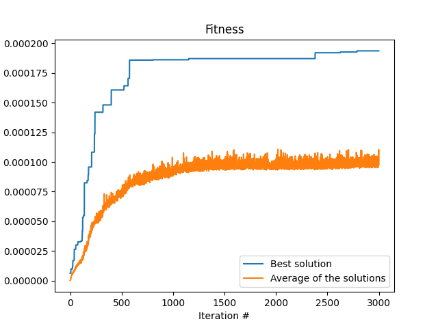
Like I wrote in the beginning, this algorithm is not the most efficient. It is after all mostly random. There are more efficient algorithms for polynomial curve fitting out there. Anyway, here are the results of the algorithm. First is the fitness as a function of the iteration number, that is, the amount of time the loop run. One can see the typical shape that we are waiting for a converging algorithm. At the start of the program, at low iteration number, the fitness is very low. But we see that there are jumps in the fitness every now and then, that indicates that the algorithm is finding better and better solutions.
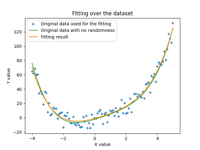
The next image shows the actual curve that we found in this run in orange, and we make the comparison with the data used to fit it with the randomness that was added (blue crosses) and actually the same data but without the randomness. We can see that the solution found by the algorithm is indeed very close to the actual data we started with. This is quite amazing.
Sources
[2] Crossing Over
The whole algorithm is in my github: https://github.com/opto-mario/genetic_algorithm