The first image from the James Webb Space Telescope (JWST) was uncover a few days ago [1]. This is truely an incredible image, showing the galactic cluster SMACS 0723, which is slowly becoming the de-facto target for newly deployed space telescopes as it was imaged by Hubble, Planck and Chandra before JWST. This image in particular took the JWST 12.5 hours of exposure to be able to see these objects as they are so dim in the sky.
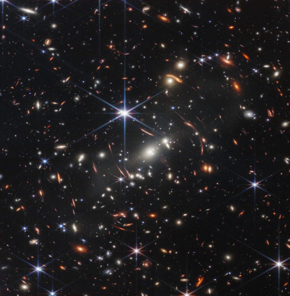
The best way to see how much of an achievement this is, is to compare it to the previous picture, taken by Hubble. Hubble’s image is not only less bright, if you zoom in, you will also notice it is less resolved and more grainy. But the big difference is the time it took to make it. Hubble took 2 weeks to make the same image, 2 whole weeks of exposure… Think about it, that is about 25 times more than the JWST, for a result that is far less impressive. Again, congratulations to the teams of the JWST for this incredible tool.
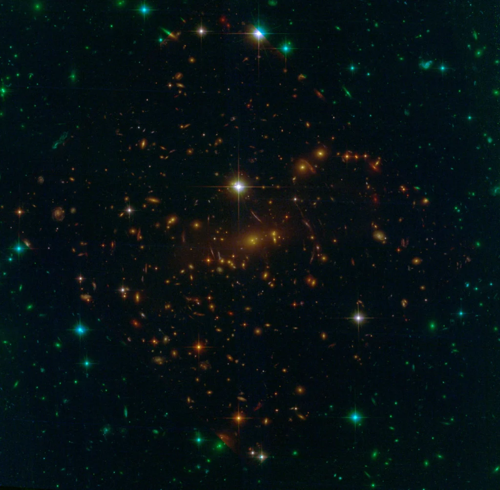
Now, the acute observer might have noticed some differences between the two images. Of course, there are more details in the JWST image, more reddish objects that were too dim or too in the infrared for Hubble to see. You can also see that both images are not perfectly in the same orientation. Also, there is some weird shading going on on the Hubble picture, which causes the objects in the center of the image to be more red and the objects on the outside more blue. But that is not what I want to focus on. What I want to focus on is the “spikes” of the stars.
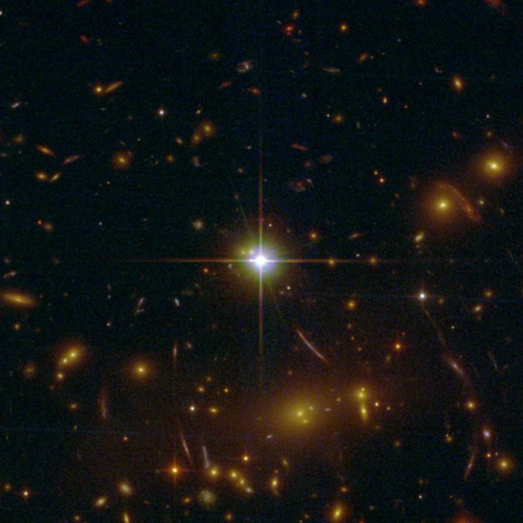
On the JWST image, the stars have all 8 spikes (6 main ones, and 2 smaller horizontal ones). On the Hubble image, they all have 4 spikes. What is going on? The answer is simple. It’s the eternal enemy of optics: diffraction.
Diffraction is inevitable. It is a consequence of the finite size of our world, the finite size of the lenses and the finite size of the sensor. Diffraction is a function of the wavelength and the size of the object that we consider that is causing the diffraction. The bigger the wavelength, the bigger the effect. The smaller the object causing diffraction, the bigger the effect as well. So diffraction is a bigger issue with small optical systems, with infrared imaging, and if there are small objects in front of the sensor.
Since we are talking about telescopes in this post, I am going to assume that the light is always colimated and coming from infinity. Also, let’s forget about colors altogether. Diffraction is wavelength dependent of course, but for the short discussion here, it is not important to consider the effects of chromatism. These simplifies things strongly. We are talking therefore only of monochromatic Fraunhofer diffraction, for the most scientifically enclined reading.
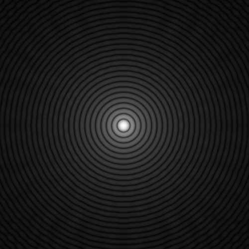
In an imaging system, everything that has an edge diffracts. Usually, the smallest elements create the strongest effect. Because most optical devices, microscopes, lenses, telescopes have a cylindrical design, the smallests elements are the appertures, which usually are circular. And the effect of that circular apperture is a diffraction pattern that looks like a series of concentric edges that is called the Airy disk. If you take an object of constant intensity, far enough so that light from this object is colimated, then this Airy disk is what the image of the object will look like in the focal plane of the optical device being used. The Airy disk is going to give you the resolution of the imaging device, as this will be the smallest point that can be focused.
Now, an interesting question is: how can we simulate these diffraction patterns? It is actually easier than it looks. All that is needed is Fourier optics. Fourier optics was really for me the moment when things clicked in my head and I saw how imaging truely works. Without going to much in the details, the idea is that when a lens makes the image of an object, we need to consider that the object can be decomposed into a sum of an infinity of objects, all of which with a sinusoidal pattern at a given frequency. This is essentially the Fourier theory applied in 2D.
So an optical device is really performing a Fourier transform over these individual objects, and the sum is going to be the actual image of the object. To simulate the diffraction pattern, all that is needed is actually to take a flat field at infinity and the apperture of the optics that you are taking into consideration and compute the Fourier transform of the aperture. The Fourier transform of a circular aperture is a Bessel function, which is actually the Airy disk, which is what you see in the Figure 4.
So let’s make the simulation of the diffractive pattern of the primary mirror from Hubble…

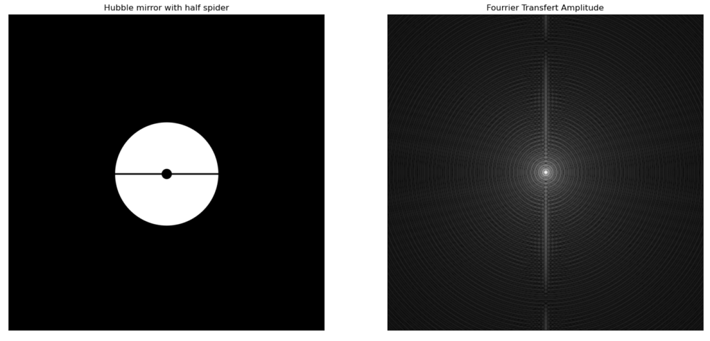
But now, let’s complicate things a little. Because in a reflective telescope, we usually need struts to hold the secondary mirror. These struts get in the way of the light, and because they are of finite size, they diffract! And their diffraction pattern adds to the existing Airy disk. By the way, these struts are called spider in telescopes building. As we can see in the picture, adding the spider leg create a line, perpendicular to the direction of the leg….
Adding another spider leg in the other direction creates the corresponding perpendicular arm line in the image.
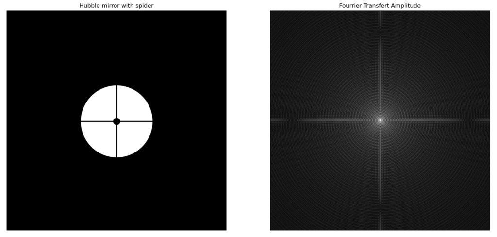
And if you look at the image from Hubble, you can see this pattern emerging actually. So you can be definitely sure that somewhere in Hubble, there is this spider hanging, holding an important optical component… And indeed, we can see that the secondary mirror of hubble is hold by a set of struts in the middle of the telescope.
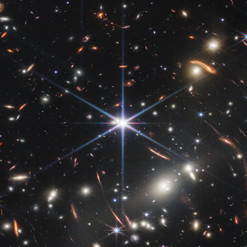
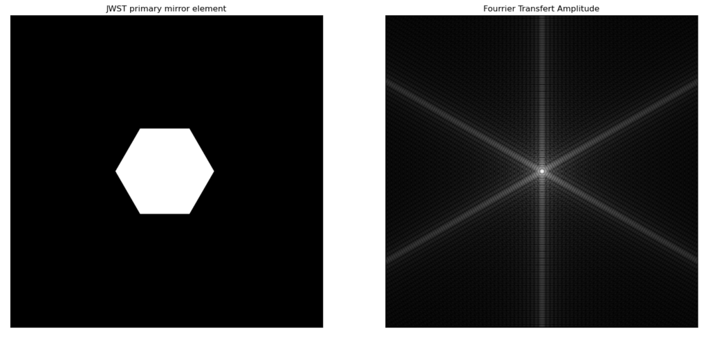
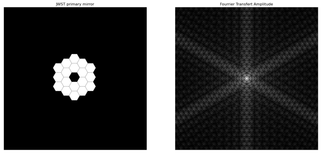
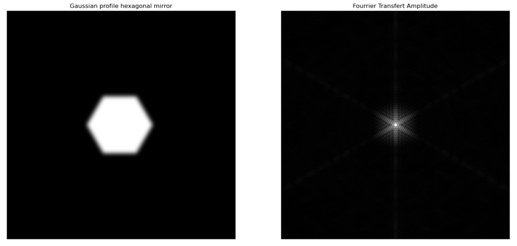
The design of the JWST is significantly different from Hubble. In particular the set of hexagonal mirrors used as primary mirror instead of the single primary mirror for Hubble. Diffraction from a single hexagonal mirror is significantly different than for a single round mirror. Because the lines are straight in the hexagonal mirror, diffraction is essentially concentrated in these directions. 3 directions to be precise, hortogonal to the direction of the edges. This makes very strong lines that we can see. But that is not all. Because the primary mirror is not just a single hexagonal mirror but a collection of smaller hexagonal mirrors, the actual diffraction pattern is slightly more pronounced and more complex. The resulting diffraction patter is as follow. You can see the complexity increasing, and looking at the image actually taken by the JWST, we are not far from it. Missing is the horizontal line. And as we saw with Hubble, these lines usually come from spiders.
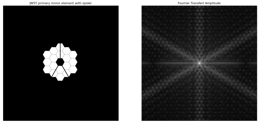
The JWST is built along the same design as hubble, in term of primary and secondary mirror. In the JWST, the secondary mirror is held by 3 struts. 2 of which are actually along the lines of the hexagonal mirror, which means that their diffraction pattern essentially blend with the diffraction pattern of the mirrors. But there is one strut that cuts the hexagonal symetry for some reason. This strut comes straight down, and is at the origin of the horizontal diffraction line. This result is really close to the actual diffraction pattern from an actual image of a star done by the JWST in figure 12. Of course, the actual image includes chromatic effect that I didn’t take into account here, and the intensity is really different, but the overall pattern is there, along with the myriad of dots that appear from the periodic arrangement of the hexagonal mirrors.

I have to say that I am quite perplexed by this decision to have this strut cutting the mirror in half and adding another diffractive line. But I am sure that the NASA engineers had no other options. The thing is that this diffraction pattern not only occurs on the stars, but really on any point in the image, making the whole thing blurrier than it could. But because the other objects are less bright, the effect is less visible, thankfully. Also, one thig to consider is that the JWST is mostly thought to observe in the infrared, where these diffractive effects will be smaller, because of the bigger wavelength than in visible light.
Still, it opens a question: how could we limit diffraction? One way is to blend the edges. Instead of having perfectly reflecting edges, having a gradient at the edge where the transition between the center of the mirror and the outside of the mirror is more gradual can help reduce the effect of the diffraction that we see here. Of course, the price to pay is a slightly lower efficiency of the whole system is term of photon collection. Depending on the amount of gradient, I assume that we could lose 2-5% of the total photons that could be captured, but then again, those photons are scattered by their proximity to the edges, and carry “false” information potentially… So… win-win?
The other drawback of this method is the fabrication process. How to modulate the reflectivity of the mirror to such degree is not easy. The mirrors of the JWST are made of a base of Berylium, polished and covered with a microscopic film of gold… A dirty and easy way would be to apply some sort of secondary opaque coating on the mirror, while the center of it is protected…. Anything that would make the mirror more lossy around the edges really.
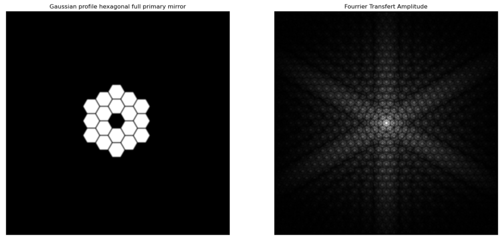
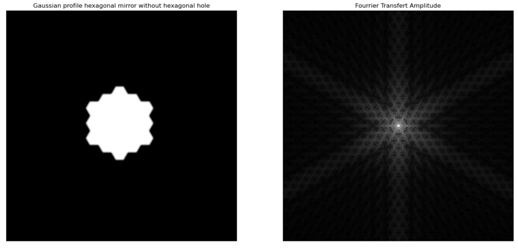
With the full JWST mirror like in figure 14, I thought at first that the pattern we see in the diffraction comes from the pseudo-periodicity of the mirrors. But this actually comes mostly from the edges of the mirror, as can be seen in figure 15.
But this still doesn’t help alleviate the effects of the spider. This is really not an easy problem… And I think NASA really did the best that could be done with today’s equipment. Congratulations to them for this amazing instrument and I look forward the discoveries this telescope will help achieve.
Code for computing the diffraction pattern in Python
import cv2
import numpy as np
from matplotlib import pyplot as plt


image_picture = "test_image.jpg"

img = cv2.imread(image_picture, 0)

# If needs to be rotated 90°
img = cv2.rotate(img, cv2.ROTATE_90_CLOCKWISE)

# Making the Fourier transform
f = np.fft.fft2(img)
fshift = np.fft.fftshift(f)
magnitude_spectrum = (20*np.log(np.abs(fshift)))**4
# I do here the power of 4 instead of 2 to have the result look more closely to what we actually get...

plt.subplot(121)
plt.imshow(img, cmap='gray')
plt.title('Gaussian profile hexagonal full primary mirror'), plt.xticks([]), plt.yticks([])


width = magnitude_spectrum.shape[0]
height = magnitude_spectrum.shape[1]
fft_width = 500
fft_height = 500

w_start = round((width-fft_width)/2)
w_end = round((width+fft_width)/2)
h_start = round((height-fft_height)/2)
h_end = round((height + fft_height)/2)

plt.subplot(122)
plt.imshow(magnitude_spectrum[w_start:w_end,h_start:h_end], cmap='gray')
plt.title('Fourrier Transfert Amplitude'), plt.xticks([]), plt.yticks([])
plt.show()
Sources
[2] https://stsci-opo.org/STScI-01G6933BG2JKATWE1MGT1TCPJ9.png
[3] https://www.nasa.gov/content/goddard/hubble-space-telescope-optics-system
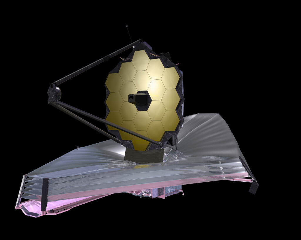
[4] https://en.wikipedia.org/wiki/James_Webb_Space_Telescope
[7] https://en.wikipedia.org/wiki/Fourier_optics
[9] https://www.nasa.gov/content/goddard/hubble-space-telescope-optics-system
[10] https://webb.nasa.gov/content/observatory/ote/mirrors/index.html